8.3.2 The jogger and the dog

We consider the following problem: a jogger is running along his favorite trail on the plane in order to get his daily exercise. Suddenly, he is being attacked by a dog. The dog is running with constant speed $w$ towards the jogger. Compute the orbit of the dog.

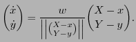
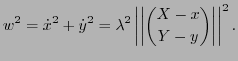
The orbit of the dog has the property that the velocity vector of the dog points at every time to its goal, the jogger. We assume that the jogger is running on some trail and that his motion is described by the two functions $X(t)$ and $Y(t)$.

Let us assume that for $t=0$ the dog is at the point  $(x_0, y_0)$, and that at time $t$ his position will be  $(x(t), y(t))$. The following equations hold:

1. $\dot{x}^2 + \dot{y}^2 = w^2$: The dog is running with constant speed.
2. The velocity vector of the dog is parallel to the difference vector between the position of the jogger and the dog:
   $${\dot{x} \choose \dot{y}} = \lambda {X-x \choose Y -y} \quad \hbox{with $\lambda>0$}.$$

If we substitute this in the first equation we obtain

$$w^2 = \dot{x}^2 + \dot{y}^2 = \lambda^2 \left \vert \left \vert {X-x \choose Y-y} \right\vert \right\vert^2.$$

This equation can be solved for $\lambda$:

$$\lambda = \frac{w}{ {\left \vert \left \vert {X-x \choose Y-y} \right\vert \right\vert} } > 0.$$

Finally, substitution of this expression for $\lambda$ in the second equation yields the differential equation of the orbit of the dog:

$${\dot{x}\choose \dot{y}} = \frac{w}{\left \vert \left \vert {X-x \choose Y-y} \right\vert \right\vert }{X-x \choose Y-y}.$$ (8.7)

Again we will make use of one of the M-files ode23.m or ode45.m to integrate the system of differential equations. We notice that the system (8.7) has a singularity when the dog reaches the jogger. In this case the norm of the difference vector becomes zero and we have to stop the integration. The above mentioned MATLAB functions for integrating differential equations require as input an interval of the independent variable. MATLAB 5.0 provides now also the possibility to define another termination criterion for the integration, different from a given upper bound for the independent variable. It is possible to terminate the integration by checking zero crossings of a function. In our example one would like to terminate integration when the dog reaches the jogger, i.e. when $\left \vert \left \vert (X-x, Y-y) \right\vert \right\vert$ becomes small. In order to do so we have to add a third input and two more output parameters to the M-function dog.m. The integrator ode23 or ode45 calls the function in two ways: The first one consists of dropping the third parameter. The function then returns only the parameter zs: the speed of the dog. In the second way the keyword 'events' is assigned to the parameter flag. This keyword tells the function to return the zero-crossing function in the first output zs. The second output isterminal is a logical vector that tells the integrator, which components of the first output force the procedure to stop when they become zero. Every component with this property is marked with a nonzero entry in isterminal. The third output parameter direction is also a vector that indicates for each component of zs if zero crossings shall only be regarded for increasing values (direction = 1), decreasing values ( direction = -1) or in both cases (direction = 0). The condition for zero crossings is checked in the integrator. The speed $w$ of the dog must be declared global in dog and in the main program. The orbit of the jogger is given by the M-function jogger.m.

function [zs,isterminal,direction] = dog(t,z,flag);
%
global w  % w = speed of the dog
X= jogger(t);
h= X-z;
nh= norm(h);
if nargin < 3 | isempty(flag) % normal output
   zs= (w/nh)*h;
else
   switch(flag)
   case 'events'  % at norm(h)=0 there is a singularity
      zs= nh-1e-3;   % zero crossing at pos_dog=pos_jogger
      isterminal= 1; % this is a stopping event
      direction= 0;  % don't care if decrease or increase
   otherwise
      error(['Unknown flag: ' flag]);
   end
end

The main program main2.m defines the initial conditions and calls ode23 for the integration. We have to provide an upper bound of the time $t$ for the integration.

   % main2.m
   global w
   y0 = [60;70];  % initial conditions, starting point of the dog
   w = 10;        % w  speed of the dog
   options= odeset('RelTol',1e-5,'Events','on');
   [t,Y] = ode23('dog',[0,20],y0,options);
   clf; hold on;
   axis([-10,100,-10,70]);
   plot(Y(:,1),Y(:,2));
   J=[];
 
   for h= 1: length(t),
      w  = jogger(t(h));
      J = [J; w'];
   end;
   plot(J(:,1), J(:,2),':');

The integration will stop either if the upper bound for the time $t$ is reached or if the dog catches up with the jogger. For the latter case we set the flag Events of the ODE options to 'on'. This tells the integrator to check for zero crossings of the function dog called with flag = 'events'. After the call to ode23 the variable Y contains a table with the values of the two functions $x(t)$ and $y(t)$. We plot the orbit of the dog simply by the statement plot(Y(:,1),Y(:,2)). In order to show also the orbit of the jogger we have to compute it again using the vector $t$ and the function jogger.

Let us now compute a few examples. First we let the jogger run along the $x$-axis:

    function s = jogger(t);
    s   = [8*t; 0];

In the above main program we chose the speed of the dog as $w=10$, and since here we have $X(t) = 8t$ the jogger is slower. As we can see the dog is catching the poor jogger.

If we wish to indicate the position of the jogger's troubles, (perhaps to build a small memorial), we can make use of the following file cross.m

      function cross(Cx,Cy,v)
      % draws at position  Cx,Cy  a cross of height 2.5v
      % and width 2*v
      Kx = [Cx Cx Cx Cx-v Cx+v];
      Ky = [Cy Cy+2.5*v Cy+1.5*v Cy+1.5*v Cy+1.5*v];
      plot(Kx,Ky);
      plot(Cx,Cy,'o');

The cross in the plot was generated by appending the statements

   p = max(size(Y));
   cross(Y(p,1),Y(p,2),2)

to the main program.

The next example shows the situation where the jogger turns around and tries to run back home:

   function s = jogger1(t);
   %
   if t<6, s = [8*t; 0];
   else    s = [8*(12-t) ;0];
   end

However, using the same main program as before the dog catches up with the jogger at time $t= 9.3$.

Let us now consider a faster jogger running on an ellipse

   function s = jogger2(t);
   s   = [  10+20*cos(t)
         20 + 15*sin(t)];

If the dog also runs fast ($w=19$), he manages to reach the jogger at time $t = 8.97$.

We finally consider an old, slow dog ($w=10$). He tries to catch a jogger running on a elliptic track. However, instead of waiting for the jogger somewhere on the ellipse, he runs (too slow) after his target, and we can see a steady state developing where the dog is running on a closed orbit inside the ellipse.