Nächste Seite: 8.4.1 Fitting two Parallel Aufwärts: 8. Anwendungen aus der Vorherige Seite: 8.3.3 Showing motion with Inhalt
Fitting a line to a set of points in such a way that the sum of squares
of the distances of the given points to the line is minimized, is known
to be related to the computation of the main axes of an inertia tensor.
Often this fact is used to fit a line and a plane to given points in the
3d space by solving an eigenvalue problem for a ![]() matrix.
matrix.
In this section we will develop a different algorithm, based on the singular value decomposition, that will allow us to fit lines, rectangles and squares to measured points in the plane and that will also be useful for some problems in 3d space.
Let us first consider the problem of fitting a straight line to a set of
given points ![]() ,
, ![]() , ...,
, ..., ![]() in the plane. We denote their
coordinates with
in the plane. We denote their
coordinates with
![]() ,
,
![]() , ...,
, ...,
![]() . Sometimes it is useful to define the vectors of
all
. Sometimes it is useful to define the vectors of
all ![]() - and
- and ![]() -coordinates. We will use
-coordinates. We will use
![]() for the vector
for the vector
![]() and similarly
and similarly
![]() for
the
for
the ![]() coordinates.
coordinates.
The problem we want to solve is not linear regression. Linear
regression means to fit the linear model ![]() to the given points,
i.e. to determine the two parameters
to the given points,
i.e. to determine the two parameters ![]() and
and ![]() such that the sum of
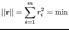
squares of the residual is minimized:
such that the sum of
squares of the residual is minimized:
 where
wherep = [ x ones(size(x))]\y; a = p(1); b = p(2);In the case of the linear regression the sum of squares of the differences of the
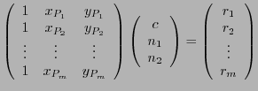
In the plane we can represent a straight line uniquely by the equations
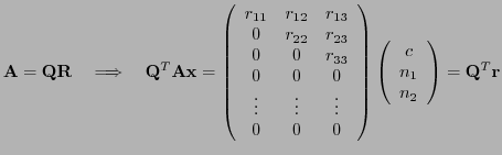
First we compute the ![]() decomposition of A and reduce our
problem to solving a small system:
decomposition of A and reduce our
problem to solving a small system:
    function [c,n] = clsq(A,dim);
    % solves the constrained least squares Problem
    % A (c n)' ~ 0 subject to norm(n,2)=1
    % length(n) = dim
    % [c,n] = clsq(A,dim)
    [m,p] = size(A);
    if p < dim+1, error ('not enough unknowns'); end;
    if m < dim, error ('not enough equations'); end;
    m = min (m, p);
    R = triu (qr (A));
    [U,S,V] = svd(R(p-dim+1:m,p-dim+1:p));
    n = V(:,dim);
    c = -R(1:p-dim,1:p-dim)\R(1:p-dim,p-dim+1:p)*n;
Let us test the function clsq with the following main program:
   % mainline.m
   Px = [1:10]'
   Py = [ 0.2 1.0 2.6 3.6 4.9 5.3 6.5 7.8 8.0 9.0]'
   A = [ones(size(Px)) Px Py]
   [c, n] = clsq(A,2)
The line computed by the program mainline has the equation
![]() . We would now like to plot the points
and the fitted line. For this we need the function plotline,
. We would now like to plot the points
and the fitted line. For this we need the function plotline,
   function plotline(x,y,s,c,n,t)
   % plots the set of points (x,y) using the symbol s
   % and plots the straight line c+n1*x+n2*y=0 using
   % the line type defined by t
   plot(x,y,s)
   xrange = [min(x) max(x)];
   yrange = [min(y) max(y)];
   if n(1)==0, % c+n2*y=0  => y = -c/n(2)
      x1=xrange(1); y1 = -c/n(2);
      x2=xrange(2); y2 = y1
   elseif n(2) == 0, % c+n1*x=0  => x = -c/n(1)
      y1=yrange(1); x1 = -c/n(1);
      y2=yrange(2); x2 = x1;
   elseif xrange(2)-xrange(1)> yrange(2)-yrange(1),
      x1=xrange(1); y1 = -(c+n(1)*x1)/n(2);
      x2=xrange(2); y2 = -(c+n(1)*x2)/n(2);
   else
      y1=yrange(1); x1 = -(c+n(2)*y1)/n(1);
      y2=yrange(2); x2 = -(c+n(2)*y2)/n(1);
   end
   plot([x1, x2], [y1,y2],t)
The picture is generated by adding the commands
   clf; hold on;
   axis([-1, 11 -1, 11])
   plotline(Px,Py,'o',c,n,'-')
   hold off;
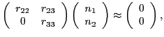 subject to