

Next: Dynamic Programming Approach
Up: Appendix
Previous: Appendix
For a tree with n different leaves, there are in the order of
 different
tree topologies [10]. If a circular order is
given, there are
O(2n-3) different trees that can be built
with that order. So a circular order alone reduces the search
space. To get an intuition we build a small table (see Table
7.1).
Figure 11:
Number of possible trees that can be built
without and with a circular order C
 |
We have seen that the probability to get a wrong TSP order is very
small. But given a correct TSP order, there are still 2n-3
possible different trees. So far we know that if the error of each
distance measurement is not larger then
 ,
where x
is the shortest edge length, we can guarantee that the tree
construction is correct.
As a next step we want to determine the
probability to get a
wrong tree for a given normal distribution of the distance
measurement. Our goal is to express the probability to get a wrong
edge in terms of the shortest edge x.
At each connection step, we connect leaf si and si+1 with
the smallest
 .
Now assume that
 has some
error s.t we connect the wrong leaves, and one of the correct
choices would have been
 .
We know that if there was
no error, then

We assume that the
 follow a normal distribution
with standard deviation
  .
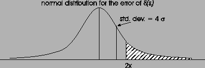
Then the error
 also follows a normal distribution
  ,
where the standard
deviation is the sum of the individual standard deviations:
 (see Figure 12).
In order to get a wrong connection, the following condition must
be true: for all
  ,
where
 is a correct
connection,
 .
This again is a normal distribution, with
 .
.
 must be
 for all
possible valid connections. For a balanced tree with n leaves
(tree depth log(n)), there are at most
 valid
connections. In the worst case, if the tree is extremely
unbalanced, there is only 1 correct connection at each step. Let
 be the probability that one
 for a given standard deviation
  :
:

So the overall probability to get a wrong connection is:
 in the best case, and
 in the worst case.
Figure:
Normal distribution for the error of

 |
To illustrate the probability to get the shortest edge x wrong
we build a table (see Table 14) for an example tree of
16 leaves. So if the standard deviation  of the error
 of the distance measurement is
  of the shortest
edge x, then the probability to get this edge wrong is
  in
the best, and
  in the worst case. Hence for very large
errors, a dynamic programming approach is more appropriate.
Figure:
Probability to get the shortest edge x
wrong depending on the standard deviation  of the error
 of the distance measurements in terms of x.
 |


Next: Dynamic Programming Approach
Up: Appendix
Previous: Appendix
Chantal Korostensky
1999-07-14


