Nächste Seite: 7.5.1 Aufgabe Aufwärts: 7. Graphik in MATLAB Vorherige Seite: 7.4 Plots mit zwei Inhalt
MATLAB kennt verschiedene Möglichkeiten, um 3D Objekte graphisch darzustellen. Den Befehl plot3 haben wir schon kennen gelernt.
Mir der Funktion mesh können 3D-Maschenflächen geplottet werden.
Zu diesem Zweck ist es von Vorteil, zunächst eine weitere Funktion
meshgrid einzuführen. Diese Funktion generiert aus zwei Vektoren
![]() (mit
(mit ![]() Elementen) und
Elementen) und ![]() (mit
(mit ![]() Elementen) ein Rechtecksgitter mit
Elementen) ein Rechtecksgitter mit
![]() Gitterpunkten.
Gitterpunkten.
    >> x = [0 1 2];
    >> y = [10 12 14];
    >> [xi yi] = meshgrid(x,y)

    xi =

         0     1     2
         0     1     2
         0     1     2


    yi =

        10    10    10
        12    12    12
        14    14    14
Der Befehl meshgrid angewandt auf die beiden Arrays
Wir können jetzt z.B. die Sattelfläche
![]() über dem Quadrat
über dem Quadrat
![]() zeichnen.
zeichnen.
    x = -1:0.05:1;
    y = x;
    [xi, yi] = meshgrid(x,y);
    zi = yi.^2 - xi.^2;
    mesh(xi, yi, zi)
    axis off
Mit
    meshc(xi, yi, zi)
    axis off
erhält man dasselbe noch mit einem Kontour-Plot.
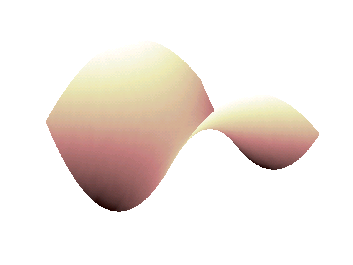
Die Maschenlinien werden als Flächen dargestellt, wenn man mesh(c) durch surf(c) ersetzt.
Die Figur 7.7 ist erhalten worden durch die Befehle
    x = -1:.05:1;  y = x;
    [xi,yi] = meshgrid(x,y);
    zi = yi.^2 - xi.^2;
    surf(xi, yi, zi)
    axis off
    colormap pink
    shading interp     % Interpolated shading
Der Befehl colormap wird verwendet um der Fläche eine bestimmte
Farbtönung zu geben. MATLAB stellt folgende Farbpaletten zur Verfügung:
| hsv | Hue-saturation-value color map (default) |
| hot | Black-red-yellow-white color map |
| gray | Linear gray-scale color map |
| bone | Gray-scale with tinge of blue color map |
| copper | Linear copper-tone color map |
| pink | Pastel shades of pink color map |
| white | All white color map |
| flag | Alternating red, white, blue, and black color map |
| lines | Color map with the line colors |
| colorcube | Enhanced color-cube color map |
| vga | Windows colormap for 16 colors |
| jet | Variant of HSV |
| prism | Prism color map |
| cool | Shades of cyan and magenta color map |
| autumn | Shades of red and yellow color map |
| spring | Shades of magenta and yellow color map |
| winter | Shades of blue and green color map |
| summer | Shades of green and yellow color map |
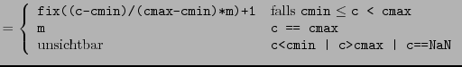
Sei m die Länge der Palette und seien cmin und cmax zwei vorgegebene Zahlen. Wenn z.B. eine Matrix mit pcolor (pseudocolor (checkerboard) plot) graphisch dargestellt werden soll, so wird ein Matrixelement mit Wert c die Farbe der Zeile ind der Palette zugeordnet, wobei
Mit dem Befehl view könnte man den Blickwinkel ändern.
Isolinien (Konturen) erhält man mit contour oder `gefüllt' mit contourf.
    x = -1:.05:1;  y = x;
    [xi,yi] = meshgrid(x,y);
    zi = yi.^2 - xi.^2;
    contourf(zi), hold on,
    shading flat               % flat = piecewise constant
    [c,h] = contour(zi,'k-');
    clabel(c,h)                % adds height labels to
                               % the current contour plot
    title('The level curves of z = y^2 - x^2.')
    ht = get(gca,'Title');
    set(ht,'FontSize',12)
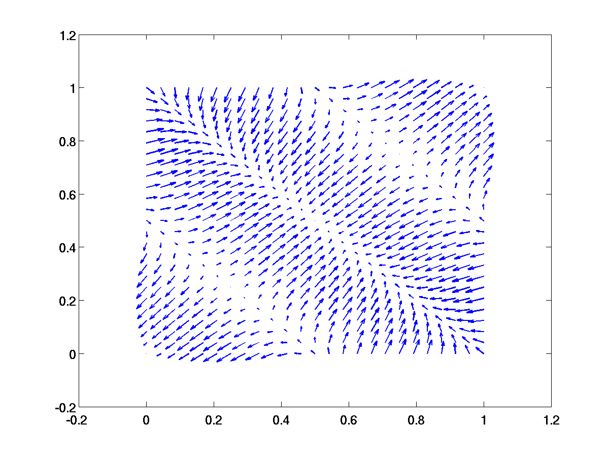
MATLAB erlaubt es auch Vektorfelder darzustellen. Wir nehmen den Gradienten der Funktion, die in Z gespeichert ist, vgl. Figur 7.8.
    >> x = [0:24]/24;
    >> y = x;
    >> for i=1:25
    >>    for j=1:25
    >>       hc = cos((x(i) + y(j) -1)*pi);
    >>       hs = sin((x(i) + y(j) -1)*pi);
    >>       gx(i,j) = -2*hs*hc*pi + 2*(x(i) - y(j));
    >>       gy(i,j) = -2*hs*hc*pi - 2*(x(i) - y(j));
    >>    end
    >> end
    >> quiver(x,y,gx,gy,1)