Let us now solve a more general problem and suppose that a child is
walking on the plane along a curve given by the two functions of
time  and
and  .
.
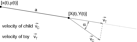
Suppose now that the child is pulling or pushing some toy,
by means of
a rigid bar of length  . We are interested in computing the orbit
of the
toy when the child is walking around.
. We are interested in computing the orbit
of the
toy when the child is walking around.
Let
 be
the position of the toy. From Figure 8.3
the following equations are obtained:
be
the position of the toy. From Figure 8.3
the following equations are obtained:
- The distance between the points
 and
is always the length of the bar. Therefore
and
is always the length of the bar. Therefore
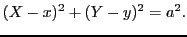 |
(8.4) |
- The toy is always moving in the direction of the bar. Therefore
the difference vector of the two positions
is a multiple of the velocity vector of the toy,
 :
:
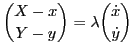 with with  |
(8.5) |
- The speed of the toy depends on the direction of the velocity
vector
 of the child. Assume, e.g., that the child is
walking on a circle of radius (length of the bar).
In this special case the toy will stay at the center of the circle
and will not move at all (this is the final state of the first
numerical example.
of the child. Assume, e.g., that the child is
walking on a circle of radius (length of the bar).
In this special case the toy will stay at the center of the circle
and will not move at all (this is the final state of the first
numerical example.
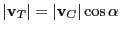
From Figure 8.3 we see that the modulus of the
velocity  of the toy is given by the modulus of the
projection of
the velocity of the child onto the bar.
of the toy is given by the modulus of the
projection of
the velocity of the child onto the bar.
Inserting Equation (8.5) into Equation (8.4), we obtain
Therefore
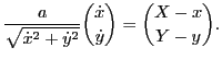 |
(8.6) |
We would like to solve Equation (8.6) for  and
and
 .
Since we know the modulus of the velocity vector of the toy
.
Since we know the modulus of the velocity vector of the toy
 , see Figure 8.3, this
can
be done by the following steps:
Now we can write the function to evaluate the system of differential
equations in MATLAB.
, see Figure 8.3, this
can
be done by the following steps:
Now we can write the function to evaluate the system of differential
equations in MATLAB.
   function zs = f(t,z)
   %
   [X Xs Y Ys] = child(t);
   v = [Xs; Ys];
   w = [X-z(1); Y-z(2)];
   w = w/norm(w);
   zs = (v'*w)*w;
The function f calls the function child which returns the
position
and velocity of the child
 for a
given time t.
As an example consider a child walking on the circle
for a
given time t.
As an example consider a child walking on the circle
 .
The corresponding function child for this
case is:
.
The corresponding function child for this
case is:
   function [X, Xs, Y, Ys] = child(t);
   %
   X  =  5*cos(t);  Y  =  5*sin(t);
   Xs = -5*sin(t);  Ys =  5*cos(t);
MATLAB offers two M-files ode23 and ode45 to integrate
differential equations.
In the following main program we will call
one of these functions and also define the initial conditions (Note
that for  the child is at the point
  and the toy
at
and the toy
at  ):
):
  % main1.m
  y0 = [10 0]';
  [t y] = ode45('f',[0 100],y0);
  clf; hold on;
  axis([-6 10 -6 10]);
  axis('square');
  plot(y(:,1),y(:,2));
If we plot the two columns of  we obtain the orbit of the toy.
Furthermore we add the curve of the child in the same plot with
the statements:
we obtain the orbit of the toy.
Furthermore we add the curve of the child in the same plot with
the statements:
   t = 0:0.05:6.3
   [X, Xs, Y, Ys] = child(t);
   plot(X,Y,':')
   hold off;
Note that the length of the bar does not appear explicitly in the
programs; it is defined implicitly by the position of the toy,
(initial condition), and the position of the child (function child) for .
Peter Arbenz
2008-09-24