Let ![]() be the number of occurrences of the variable xin the algebraic expression for f(x).
We will not take into account simplification for the time being,
we will just consider the number of occurrences as they
appear in the expression as it is written.
E.g.
be the number of occurrences of the variable xin the algebraic expression for f(x).
We will not take into account simplification for the time being,
we will just consider the number of occurrences as they
appear in the expression as it is written.
E.g.
![]() ,
whereas
,
whereas
![]() Of course, any equation for which
Of course, any equation for which ![]() is trivial to solve by
algebraic isolation,
if we know the inverses of all the functions used, even if there are
multivalue issues.
The cases where
is trivial to solve by
algebraic isolation,
if we know the inverses of all the functions used, even if there are
multivalue issues.
The cases where ![]() are considered trivial and we will now
study the case of
are considered trivial and we will now
study the case of
![]() exclusively.
exclusively.
It is easy to see, that if ![]() ,
then by algebraic isolation of
each of the occurrences of x we can usually compute kiterators of the form x = F(x) derived from f(x)=0.
Except for multivalued functions or principal values,
all of these iterators will have the same solution set as the
original1.
At this point we will not perform any simplification or any
additional manipulation to obtain the iterators.
For each occurrence of x we simply isolate it.
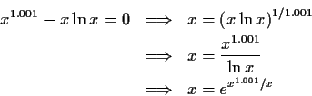
For example, from
,
then by algebraic isolation of
each of the occurrences of x we can usually compute kiterators of the form x = F(x) derived from f(x)=0.
Except for multivalued functions or principal values,
all of these iterators will have the same solution set as the
original1.
At this point we will not perform any simplification or any
additional manipulation to obtain the iterators.
For each occurrence of x we simply isolate it.
For example, from
![]() we obtain 3 iterators, namely
we obtain 3 iterators, namely
We are now ready to describe the heuristic algorithm. For f(x)=0 we compute all the iterators generated by isolation, F1(x), F2(x), ..., Fk(x). For each initial value x0 we try all the iterators a limited number of times. This is done according to the following procedure
  for x[0] in set_of_initial_values do
      for m = 1 to k do
          for i = 1 to maximum_iterations do
              x[i] := F[m](x[i-1]);
              if computation_failed or outside_domain(x[i])
                   then next m
              else if convergence_achieved
                   then return x[i]
              else if i>3 and diverging
                   then break
              else if acceleration_possible
                   then x[i] := acceleration(x[i],x[i-1],...)
              end if
          end for i
      end for m
  end for set_of_initial_values;
The idea behind this heuristic is that while it is extremely improbable that all of the iterators will converge, it is also improbable that all of them will fail to converge. By keeping the cost of running each one low, we can try all of them, expecting at least one to succeed. In practice, this heuristic is highly successful even for contrived, ill-behaved examples.