The last step

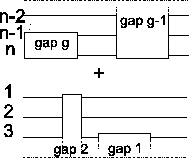
We continue this process until all n sequences are in the MSA. We have shown that the partial score of the MSA is optimal. The score $F(\mbox{\rm A})$ differs from the partial score only in the last term in the sum. The last term comes from scoring the last sequence a_n with the first sequence a₁ in the MSA. The problem is that in the algorithm we never aligned s_n with s₁ to obtain an optimal pairwise alignment, hence this score may not be optimal.

  

Figure 10: The alignment between sequences a₁ and a_n might not be optimal

Lower bound Our algorithm guarantees a lower bound $L(\mbox{\rm A})$ of least $\frac{n-1}{n}\cdot opt$ (where opt is the maximum possible score): $L(\mbox{\rm A}) \geq \frac{n-1}{n} \cdot opt$ The reason why we choose a place to cut the circle where the sequences are distant is the following: the score of the pairwise alignment that has the smallest score (in $C(\mbox{\rm A})$) adds the smallest amount to the overall sum. Since this is the only pairwise alignment that is not optimal within the MSA, we get the greatest possible lower bound $L(\mbox{\rm A})$. Hence the lower bound is $L(\mbox{\rm A}) = \frac{n-1}{n} \cdot opt$ when all the pairwise scores are the same, and it is greater otherwise. Our algorithm so far had to invest O(n k²) time for the circular alignment (where k is the length of the longest sequence) and O(n² k²) time to compute all pairwise alignments at the beginning, which is the most expensive part. Of course the TSP is exponential in n, but in real cases the calculation of the TSP order takes only a fraction of the computation time compared to the time it takes to construct the score matrix of the $n \choose{2}$ pairwise alignments. Further improvements At this point we could consider the following possibilities:

• Do nothing: in most cases the score is close enough to the optimal that we do not need to make any adjustments.
• Use a heuristic that shifts the gap blocks around to come closer to the optimum.
• Use an exhaustive algorithm to shift gap blocks around.

If we want to optimize this alignment the first thing we consider is: whatever we change, the score between the first n-1 alignments within the MSA can only get worse, since they are optimal. The only possible improvement would be to increase the score of the last alignment more than to decrease the scores of all the other alignments. This makes the search for an optimal alignment simple: we only have to consider alignments in the search where the last pairwise alignment n increases, and discard all other cases.
We show that it is very unlikely that we have to insert a gap anywhere in order to improve the alignment. Since all the pairwise alignments within the MSA are optimal except for the alignment of the last with the first sequence, any gaps we insert will decrease the score. So the only possible place where we could insert a gap in order to increase the score is either in sequence a₁ or a_n (and not both, as this would not affect the alignment $\langle a_1, a_n\rangle$):

  

Figure 11: Insertion of gap g in sequence a₁ or a_n results in an insertion of gaps in all other sequences. The score of the MSA is affected at four places (clouds)

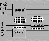
But if we insert a gap g in either sequence a_n or a₁, we have to insert another gap g' in all other sequences, otherwise some sequences in the MSA would be longer than others (see Figure 11). The score of the previously optimal alignment $\langle a_1,a_2\rangle$ is now lower by the cost of two gaps (see Figure 11). In addition, the alignment $\langle a_n, a_1\rangle$ has two additional gaps. Hence the score of the MSA could only improve, if the alignment $\langle a_1, a_n\rangle$ has now a score that is at least four times a gap cost greater than it was before. Note that the gap cost is usually very low compared to the score of aligning two amino acids. In our case the fixed gaps cost is around -14, and the score of aligning two Ala is 2.4 (depending on the PAM distance) [6,10]. So it is very unlikely that the alignment $\langle a_1, a_n\rangle$ gets better after inserting two gaps. In addition, this situation is very easy to check: we simply subtract the score of the alignment $\langle a_1, a_n\rangle$ from the optimal score OPA(s₁, s_n). If the difference is smaller than the cost of four gaps, we know for sure that we do not have to insert a gap - otherwise the alignment $\langle a_1, a_n\rangle$ could not improve by four gaps. 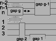Optimizing the border blocks First we need to consider where the score changes when gap blocks are moved. Let us look at the gap block with the label gap g as an example in Figure 12. If we move this gap block to the right, the score of the overall alignment is affected at exactly two places: the score between the pairwise alignment $\langle a_{n-2}, a_{n-1}\rangle$ changes, and the score on the other side of the gap block of the alignment $\langle a_n, a_1\rangle$ changes. The rest of the alignment is not disturbed. This also means that the gap blocks do not influence each other, unless they end at the same place.

  

Figure 12: The movement of a gap block only affects two places in the alignment.

We call gap blocks that end in either sequence a₁ or a_n border blocks. The only way to improve the last pairwise alignment is to move border blocks around. But whenever we move a gap block, we also disturb one optimal alignment somewhere between sequences a₁ and a_n where the border block ends. But it is possible that moving gap border blocks around will increase the score of the last alignment more than it will decrease the overall score of the alignment. The most promising optimization to do would be to remove a border block by joining border blocks that are cut apart like the ones in Figure 13. This way we remove two times the cost of a gap for each border block, and at the same time the optimal alignments of the neighboring sequences are only disturbed at one place per block (see Figure 13). To do this we only consider border blocks of same size, because if we take border blocks of different size, there would still be a gap left.

  

Figure 13: Before the optimization there are four border blocks. After shifting, two optimal alignments are disturbed a bit, but in exchange two gap blocks are gone.

If there are several bordering gap blocks of same size we need to invest some brute force searching, which is exponential in the number of bordering gap blocks: if there are b bordering gap blocks it would take in the order of O(k^b) time to compute all possibilities. However, in real cases, it does not make sense to move one gap block from one end to the complete other end of the alignment, if we assume that most gap blocks are more or less placed correctly within a certain distance. So using heuristics this complexity can further be reduced. But even without the above optimization we already have an MSA close to the optimum. 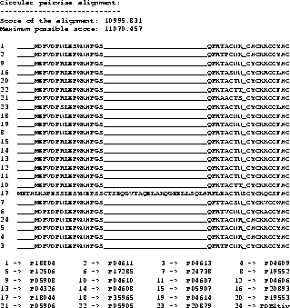Example To show a real example we took the tat protein from several strains of the Human Immunodeficiency Virus type 1 (HIV-1). The first alignment was calculated using Clustal W [35], the second one using our new algorithm, including shifting of the border blocks. Due to the size of the MSAs, only a part is shown where the results obtained by the two methods differ. The scores are determined using the CS measure. The maximum possible score in the example is the score determined using the CS measure but using the OPAs: it is the sum of the OPAs in circular order (the upper bound for the MSA A, see [11]).

The score obtained with the new algorithm is slightly better than the score obtained from Clustal W. It is clearly better at the beginning (if you ask an expert biologist), because the alignment has only one big gap whereas the alignment obtained from Clustal W has two gaps. With the above example we do not want to prove that our method performs generally better than Clustal W, but we want to show that our method is usable and produces good results. Discussion Our algorithm produces an MSA that has a score of at least $\frac{n-1}{n}\cdot opt$, where opt is the maximum possible score. It takes in the order O(n² k²) time given a circular tour. The calculation of such a tour using a TSP algorithm can be done very efficiently, and in realistic cases the calculation time of a TSP cycle can be ignored. The alignment can then further be improved using an exact or heuristic algorithm. A further advantage of this algorithm is that it does not need to calculate an evolutionary tree but uses a scoring function that takes such a tree into account. Acknowledgements We would like to thank Todd Wareham for various references and Ulrike Stege for reading the paper.