Nächste Seite: 8.5 Beispiel Prototyping: Update Aufwärts: 8.4 Fitting Lines, Rectangles Vorherige Seite: 8.4.2 Fitting Orthogonal Lines Inhalt

% rectangle.m
clf; hold on;
axis([0 10 0 10])
axis('equal')
p=100; q=100; r=100; s=100;
disp('enter points P_i belonging to side A')
disp('by clicking the mouse in the graphical window.')
disp('Finish the input by pressing the Return key')
[Px,Py] = ginput(p); plot(Px,Py,'o')
disp('enter points Q_i for side B ')
[Qx,Qy] = ginput(q); plot(Qx,Qy,'x')
disp('enter points R_i for side C ')
[Rx,Ry] = ginput(r); plot(Rx,Ry,'*')
disp('enter points S_i for side D ')
[Sx,Sy] = ginput(s); plot(Sx,Sy,'+')
zp = zeros(size(Px)); op = ones(size(Px));
zq = zeros(size(Qx)); oq = ones(size(Qx));
zr = zeros(size(Rx)); or = ones(size(Rx));
zs = zeros(size(Sx)); os = ones(size(Sx));
A = [ op zp zp zp Px Py
zq oq zq zq Qy -Qx
zr zr or zr Rx Ry
zs zs zs os Sy -Sx]
[c, n] = clsq(A,2)
% compute the 4 corners of the rectangle
B = [n [-n(2) n(1)]']
X = -B* [c([1 3 3 1])'; c([2 2 4 4])']
X = [X X(:,1)]
plot(X(1,:), X(2,:))
% compute the individual lines, if possible
if all([sum(op)>1 sum(oq)>1 sum(or)>1 sum(os)>1]),
[c1, n1] = clsq([op Px Py],2)
[c2, n2] = clsq([oq Qx Qy],2)
[c3, n3] = clsq([or Rx Ry],2)
[c4, n4] = clsq([os Sx Sy],2)
% and their intersection points
aaa = -[n1(1) n1(2); n2(1) n2(2)]\[c1; c2];
bbb = -[n2(1) n2(2); n3(1) n3(2)]\[c2; c3];
ccc = -[n3(1) n3(2); n4(1) n4(2)]\[c3; c4];
ddd = -[n4(1) n4(2); n1(1) n1(2)]\[c4; c1];
plot([aaa(1) bbb(1) ccc(1) ddd(1) aaa(1)], ...
[aaa(2) bbb(2) ccc(2) ddd(2) aaa(2)],':')
end
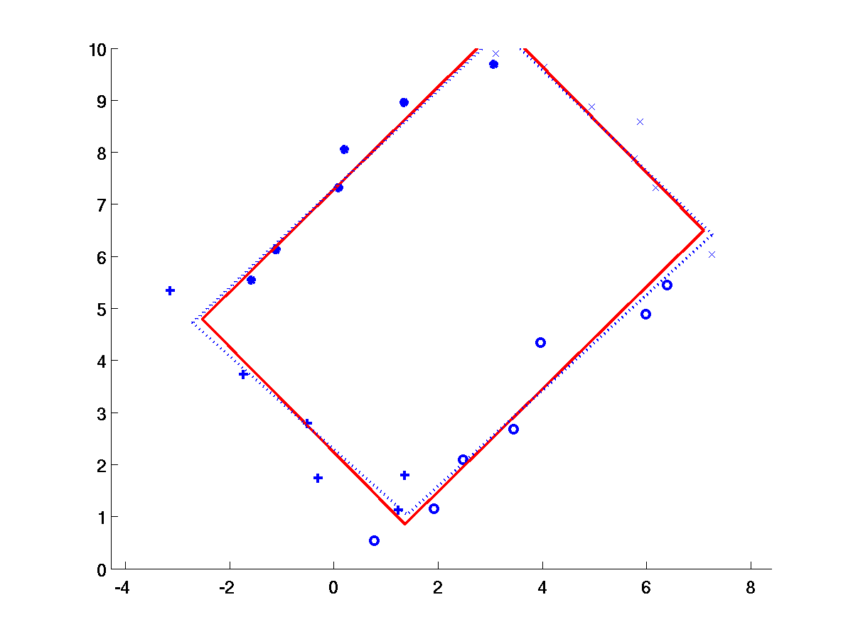
hold off;
The Program rectangle not only computes the rectangle but also fits the individual lines to the set of points. The result is shown as Figure 8.4. Some comments may be needed to understand some statements. To find the coordinates of a corner of the rectangle, we compute the point of intersection of the two lines of the corresponding sides. We have to solve the linear system

X = -B* [c([1 3 3 1])'; c([2 2 4 4])'].